
3.5 Static Forces in Manipulator
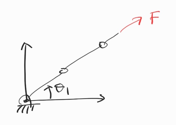
3.5.1 1 DOF Manipulator
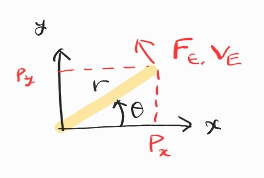
이 manipulator는 하나의 joint를 가지고 있다. 이 joint에 어떤 torque가 가해져서 움직였다고 하자. End-effector position은
\[{}^{0}P_x = x = r \cos \theta \\ {}^{0}P_y = y = r \sin \theta \\\]속도는 position을 시간에 대해 미분해서,
\[{}^{0}V_x = {}^{0}\dot{P}_x = \dot{x} = - \dot{\theta}r \sin \theta = -\omega r \sin \theta \\ {}^{0}V_y = {}^{0}\dot{P}_y = \dot{y} = \dot{\theta}r \cos \theta = \omega r \cos \theta \\\]Matrix form으로 나타내면 Jacobian을 얻는다.
\[\dot{\textbf{x}} = \textbf{J}(\boldsymbol{\theta})\dot{\boldsymbol{\theta}}\] \[\begin{bmatrix} \dot{x} \\ \dot{y} \end{bmatrix} = \begin{bmatrix} -r\sin \theta \\ r\cos\theta \end{bmatrix} \begin{bmatrix} \dot{\theta} \end{bmatrix} = \begin{bmatrix} -r\sin \theta \\ r\cos\theta \end{bmatrix} \begin{bmatrix} \omega \end{bmatrix}\]여기까지는 항상 했던 것.
3.5.2 Force Transformation
External force와 평형을 이루기 위해 joint에 가해져야 하는 torque의 크기는?
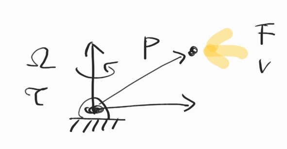
Velocity와 force를 비교해보면 뭔가 유사한 점이 있는 것 같다. 둘 다 cross product로 표현이 가능했다.
\[\begin{align*} \textbf{v} &= \boldsymbol{\Omega} \times \textbf{p} \\ \boldsymbol{\tau} &= \textbf{p} \times \textbf{F} \end{align*}\]Duality를 이루고 있는 건 아닐까?
3.5.3 Virtual Work Theorem
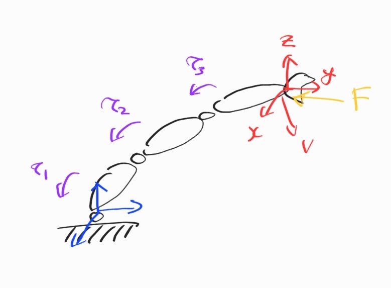
Massless, frictionless manipulator를 가정. End effector에 $\textbf{F}$에 힘이 가해진다고 하자.
Joint torque와 이에 따른 joint displacement의 내적으로부터 joint가 한 일의 양이 나온다.
반면 end-effector force과 이에 따른 displacement로부터 역시 일을 얻는다.
\[\textbf{F} \cdot \delta \textbf{x} = \boldsymbol{\tau} \cdot \delta \boldsymbol{\theta}\] \[\textbf{F}^T \delta \textbf{x} = \boldsymbol{\tau}^T \delta \boldsymbol{\theta}\]$\delta \textbf{x}$와 $\delta \boldsymbol{\theta}$가 꽤 작으면 각각 속도로 근사시킬 수 있다. 이 경우 둘 사이의 관계가 Jacobian으로 나타난다. 위 3.5.1 참조.
\[\delta \textbf{x} = \textbf{J}\delta \boldsymbol{\theta}\] \[\textbf{F}^T\textbf{J}\delta \boldsymbol{\theta} = \boldsymbol{\tau}^T \delta \boldsymbol{\theta}\] \[\textbf{F}^T\textbf{J} = \boldsymbol{\tau}^T\]따라서 우리는 velocity transformation으로부터 force transformation을 얻을 수 있다.
\[\dot{\textbf{x}} = \textbf{J}(\boldsymbol{\theta})\dot{\boldsymbol{\theta}} \qquad \Rightarrow \qquad \boldsymbol{\tau} = \textbf{J}^T\textbf{F}\]3.5.4 Proterties of Jacobian
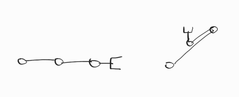
3D planar manipulator를 예시로 들자.
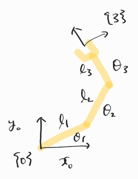
Jacobian의 determinant를 구하면 다음과 같다.
\[\textrm{det}(\textbf{J}(\boldsymbol{\theta})) = \begin{vmatrix} -(l_1s_1 + l_2s_{12} + l_3s_{123} & -(l_2s_{12}+l_3s_{123}) & -l_3s_{123} \\ l_1c_1 + l_2c_{12} + l_3c_{123} & l_2c_{12}+l_3c_{123} & l_3c_{123} \\ 1 & 1 & 1 \end{vmatrix} = l_1l_2s_2\]$\textrm{det}(\textbf{J}(\boldsymbol{\theta}))$가 $\theta_1, \theta_3$의 함수가 아님에 주목. $\textrm{det}$가 $0$이 되는 $\theta_2$는 $0$ 또는 $\pi$이다.
Singular configuration!
Joint torque와 end effector force의 관계는
\[\boldsymbol{\tau} = \textbf{J}^T(\boldsymbol{\theta})\textbf{F}\]$\textbf{J}^T$의 rank는 $\textbf{J}$와 같다. Singular configuration에서는 어떤 non-trivial force $\textbf{F}$가 존재해서,
\[\boldsymbol{\tau} = \textbf{J}^T(\boldsymbol{\theta})\textbf{F} = \textbf{0}\]을 만족하게 된다. 즉 어떤 유한한 force가 end effector에 작용했으나 robot joint에 어떤 torque도 만들어내지 않는 case. Manipulator가 locked up된 것.
예시 중 하나. $\theta_1=\theta$, $\theta_2 = \theta_3 = 0$이고, end effector에 가해지는 힘이
\[{}^{0}\textbf{F} = \begin{bmatrix} Fc_1 \\ Fs_1 \\ 0 \end{bmatrix}\]인 경우.
위에 구해 놓은 Jacobian을 이용해 계산하면 실제로 ${}^{0} \boldsymbol{\tau} = \textbf{0}$을 얻을 수 있다.
3.5.5 Velocity and Force Transformation
Body의 general velocity $\boldsymbol{\nu}$를 $6 \times 1$로 표현했었다.
\[\boldsymbol{\nu} = \begin{bmatrix} v \\ \omega \end{bmatrix}\]비슷하게, general force vector를 $6 \times 1$로 표현할 수 있을 것 같다.
\[\mathcal{F} = \begin{bmatrix} F \\ N \end{bmatrix}\]여기서 $F$는 $3 \times 1$ force vector, $N$는 $3 \times 1$ moment vector이다. 그러면 자연스럽게 한 frame으로부터 다른 frame의 $6 \times 6$ transformation도 생각할 수 있겠다.
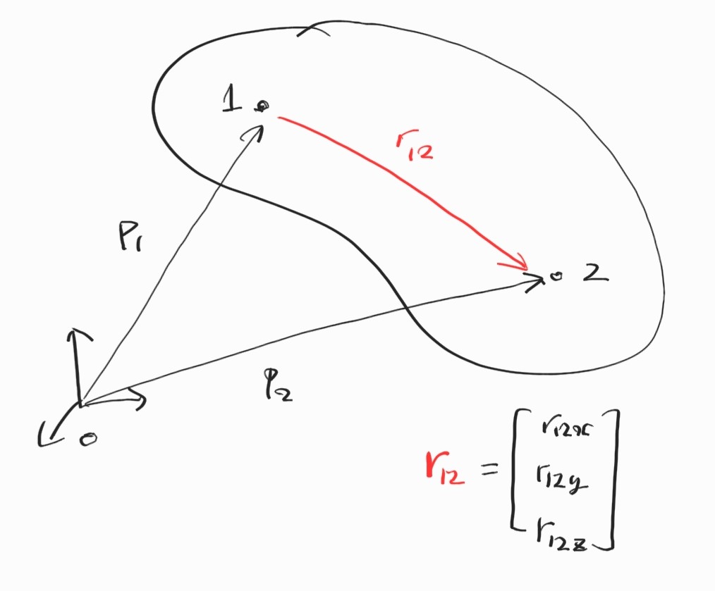
Single rigid body에 대해,
\[\boldsymbol{\omega}_2 = \boldsymbol{\omega}_1 \\ \dot{\textbf{p}}_2 = \dot{\textbf{p}}_1 + \boldsymbol{\omega}_1 \times \textbf{r}_{12}\]Cross product를 skew-symmetric matrix로 표현하면 다음과 같이 정리된다.
\[\begin{bmatrix} \dot{\textbf{p}}_2 \\ \boldsymbol{\omega}_2 \end{bmatrix} = \begin{bmatrix} \textbf{I} & -\textbf{S}(\textbf{r}_{12}) \\ \textbf{0} & \textbf{I} \end{bmatrix} \begin{bmatrix} \dot{\textbf{p}}_1 \\ \boldsymbol{\omega}_1 \end{bmatrix}\]이것으로 single rigid body 위의 두 점에서의 velocity transform 완성.
Gripper에 가해지는 힘의 크기를 측정하고 싶다고 하자. Gripper가 벽에 닿는 부분에 sensor를 바로 부착할 수는 없으니 sensor가 달린 link에 rigid하게 gripper를 부착하자.
이제, sensor가 측정한 force로부터 gripper가 받는 힘을 알아내야 한다.
먼저 속도부터. 위 single rigid body case를 이용한다. Sensor의 좌표계를 $\{A \}$, gripper의 좌표계를 $\{B \}$로 두면, rotational matrix를 추가해
\[\begin{bmatrix} {}^{B} \textbf{v}_B \\ {}^{B} \boldsymbol{\omega}_B \end{bmatrix} = \begin{bmatrix} {}^{B}\textbf{R}_A & -{}^{B}\textbf{R}_A[{}^{A}\textbf{P}_{BORG}^{\times}] \\ \textbf{0} & {}^{B}\textbf{R}_A \end{bmatrix} \begin{bmatrix} {}^{A}\textbf{v}_A \\ {}^{A}\boldsymbol{\omega}_A \end{bmatrix}, \qquad [\textbf{P}^{\times}] = \begin{bmatrix} 0 & -p_z & p_y \\ p_z & 0 & -p_x \\ -p_y & p_x & 0 \end{bmatrix}\]마지막으로 force transformation.
\[\begin{bmatrix} {}^{A} \textbf{F}_A \\ {}^{A} \textbf{N}_A \end{bmatrix} = \begin{bmatrix} {}^{A}\textbf{R}_B & \textbf{O} \\ [{}^{A}\textbf{P}_{BORG}^{\times}]{}^{A}\textbf{R}_B & {}^{A}\textbf{R}_B \end{bmatrix} \begin{bmatrix} {}^{B} \textbf{F}_B \\ {}^{B} \textbf{N}_B \end{bmatrix}\]