
3.4 Differential Kinematics in 3D (3)
3.4.1 Singular Value Decomposition
Jacobian matrix는 다음 세 행렬의 곱으로 나타낼 수 있다.
\[\textbf{J}(\textbf{q}) = \textbf{U}\boldsymbol{\Sigma}\textbf{V}^T\]여기서 $\textbf{U} \in \mathbb{R}^{m \times m}$, $\textbf{V} \in \mathbb{R}^{n \times n}$은 orthogonal matrix이며,
\[\boldsymbol{\Sigma} = \textrm{diag}(\sigma_1, \sigma_2, \cdots , \sigma_m) \\ \sigma_1 \geq \sigma_2 \geq \cdots \geq \sigma_n\]3.4.2 Velocity Ellipsoid in 3D
기본 내용은 2D일 때와 같다. Unit norm을 가지는 모든 joint velocity들의 set에서,
\[\Vert \dot{\boldsymbol{\theta}} \Vert^2 = \dot{\boldsymbol{\theta}} \cdot \dot{\boldsymbol{\theta}} = \dot{\boldsymbol{\theta}}^T\dot{\boldsymbol{\theta}} = 1 \\ \dot{\boldsymbol{\theta}} = \textbf{J}^{-1} \boldsymbol{\nu} \\ \boldsymbol{\nu}^T(\textbf{J}\textbf{J}^T)\boldsymbol{\nu} = 1\]이 방정식은 6D hyper ellipsoid equation이 된다.
Velocity ellipsoid는 어떤 정보를 줄까?
로봇은 longest axis direction(largest singular value)를 따라 가장 빠르게 움직이며, shortest axis direction(smallest singular value)를 따라 가장 천천히 움직인다.
Ellipsoid가 sphere이면, motion은 isotropic하며 모든 방향에서 동일한 속도를 갖는다.
3.4.3 Manipulability
Manipulability는 ellipsoid의 크기로 정의된다.
\[m = \sqrt{\textrm{det}(\textbf{J}\textbf{J}^T)} = \sigma_1 \cdot \sigma_2 \cdots \sigma_m\]여기서 $\sigma_1, \sigma_2, \cdots , \sigma_m$은 Jacobian의 singular value.
Ellipsoid의 condition number는 ellipsoid의 형태를 나타내는 수이다.
\[\kappa = \frac{\sigma_1}{\sigma_m}, \qquad 1 \leq \kappa\]$m=1$이면 robot은 isotropic motion을 한다. $m= \infty$이면 ellipsoid는 단순한 ellipse가 된다. 이 경우 Cartesian 방향의 motion이 불가능해진다.
3.4.4 Transforming Spatial Velocity
2D case에서 Jacobian을 통해 frame 사이의 velocity transformation을 진행했다. 3D에서도 예외는 아니다.
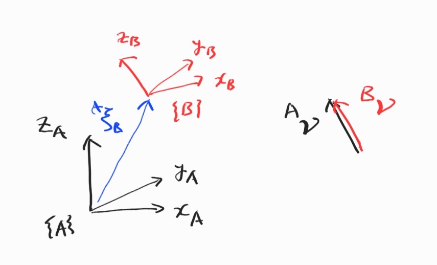
2D case였던 3.1.5와 비교해보자.
이제 world coordinate frame $\{0 \}$에서 spatial velocity는
\[\begin{align*} {}^{0}\boldsymbol{\nu} &= {}^{0}\textbf{J} \dot{\boldsymbol{\theta}} \\ {}^{6}\boldsymbol{\nu} &= {}^{6}\textbf{J} \dot{\boldsymbol{\theta}} \\ &= {}^{6}\textbf{J}_0({}^{6}\xi_0){}^{0}\textbf{J}(\boldsymbol{\theta})\dot{\boldsymbol{\theta}} \end{align*}\] \[{}^{6}\textbf{J}_0({}^{6} \xi_0) = \begin{bmatrix} {}^{6} \textbf{R}_0 & \textbf{0}_{3 \times 3} \\ \textbf{0}_{3 \times 3} & {}^{6} \textbf{R}_0 \end{bmatrix}\]3.4.5 Rate of Euler Angles
지금까지 열심히 Jacobian으로 spatial velocity를 계산했는데, 생각해 보면 우리는 지금까지 각도를 Euler angle로도 표현해왔다.
실제로 물체는 Euler angle을 따라 회전하는 것이 아니다. Euler angle은 그저 각도를 기술하기 위해 우리가 적당히 정한 것이었다.
$ZYZ$ Euler angle rate를 실제 각속도로 바꾸려면?
\[\boldsymbol{\Omega}_{ZYZ} = \begin{bmatrix} \dot{\alpha} \\ \dot{\beta} \\ \dot{\gamma} \\ \end{bmatrix}, \qquad \boldsymbol{\omega} = \begin{bmatrix} \omega_x \\ \omega_y \\ \omega_z \\ \end{bmatrix}\]3.2.7을 참조. Skew-symmetric matrix
\[\textbf{S} = \dot{\textbf{R}}\textbf{R}^T = \begin{bmatrix} 0 & -\omega_z & \omega_y \\ \omega_z & 0 & -\omega_x \\ -\omega_y & \omega_x & 0 \end{bmatrix}\]여기서 세 independent equation을 가져올 수 있다.
\[\begin{align*} \omega_x &= \dot{r_{31}}r_{21} + \dot{r_{32}}r_{22} + \dot{r_{33}}r_{23} \\ \omega_y &= \dot{r_{11}}r_{31} + \dot{r_{12}}r_{32} + \dot{r_{13}}r_{33} \\ \omega_z &= \dot{r_{21}}r_{11} + \dot{r_{22}}r_{12} + \dot{r_{23}}r_{13} \\ \end{align*}\]이제 Euler-angle rate와 angular velocity 사이의 관계를 구하자. 다음과 같이 표현.
\[\boldsymbol{\omega} = \textbf{K}(\alpha, \beta, \gamma) \boldsymbol{\Omega}_{ZYZ}\]즉, 여기서 $\textbf{K}(\alpha, \beta, \gamma)$는 둘 사이의 Jacobian이 된다.
$ZYZ$ Euler angle의 Rotation matrix는… 1.3.2에 있었다.
\[\begin{align*} {}^{A}\textbf{R}_B &= \textbf{R}_Z(\alpha)\textbf{R}_Y(\beta)\textbf{R}_Z(\gamma) \\ &= \begin{bmatrix} \cos \alpha & -\sin \alpha & 0 \\ \sin \alpha & \cos \alpha & 0 \\ 0 & 0 & 1 \end{bmatrix} \begin{bmatrix} \cos \beta & 0 & \sin \beta \\ 0 & 1 & 0 \\ -\sin \beta & 0 & \cos \beta \end{bmatrix} \begin{bmatrix} \cos \gamma & -\sin \gamma & 0 \\ \sin \gamma & \cos \gamma & 0 \\ 0 & 0 & 1 \end{bmatrix} \end{align*}\]위를 계산해서 풀든 또는 실제로 회전시켜가며 좌표계가 어떻게 옮겨가는지를 확인하든, 다음을 얻을 수 있다.
\[\textbf{K}(\alpha, \beta, \gamma) = \begin{bmatrix} 0 & -\sin\alpha & \cos\alpha\sin\beta \\ 0 & \cos\alpha & \sin\alpha\sin\beta \\ 1 & 0 & \cos\beta \end{bmatrix}\]이제 직관적으로 정리할 수 있겠다.
\[\boldsymbol{\nu} = \textbf{J}(\boldsymbol{\theta})\boldsymbol{\theta} \qquad \boldsymbol{\nu} = \begin{bmatrix} v_x & v_y & v_z & \omega_x & \omega_y & \omega_z \end{bmatrix}^T \\ \boldsymbol{\nu}_e = \textbf{J}_e(\boldsymbol{\theta})\boldsymbol{\theta} \qquad \boldsymbol{\nu}_e = \begin{bmatrix} v_x & v_y & v_z & \alpha & \beta & \gamma \end{bmatrix}^T \\\] \[\textbf{J}_e(\boldsymbol{\theta}) = \begin{bmatrix} \textbf{I}_{3 \times 3} & \textbf{0}_{3 \times 3} \\ \textbf{0}_{3 \times 3} & \textbf{K}^{-1}(\alpha, \beta, \gamma) \end{bmatrix} \textbf{J}(\boldsymbol{\theta})\]3.4.6 Rate of Quaternion
Quaternion도 있었지. $q = q_0+iq_1+jq_2+kq_3 = (q_0,q_1,q_2,q_3)$ 이라고 하면, quaternion rate와 rotation vector 사이의 관계는
\[\dot{q} = \begin{bmatrix} q_0 \\ q_1 \\ q_2 \\ q_3 \end{bmatrix} = \frac{1}{2} \begin{bmatrix} q_0 & -q_1 & -q_2 & -q_3 \\ q_1 & q_0 & -q_3 & q_2 \\ q_2 & q_3 & q_0 & -q_1 \\ q_3 & -q_2 & q_1 & q_0 \\ \end{bmatrix} \begin{bmatrix} 0 \\ \omega_x \\ \omega_y \\ \omega_z \end{bmatrix}\]유도는 생략.
3.4.7 Shape of Jacobian
Jacobian은 joint 하나 당 한 column. 총 $N$-개 column을 가진다. 하나의 row는 spatial velocity 성분으로, 3D motion의 경우 6개의 row가 있다.
\[\begin{bmatrix} v_x \\ v_y \\ v_z \\ \omega_x \\ \omega_y \\ \omega_z \end{bmatrix} = \textbf{J}(\boldsymbol{\theta}) \begin{bmatrix} \dot{\theta}_1 \\ \dot{\theta}_2 \\ \vdots \\\dot{\theta}_N \end{bmatrix} \qquad \textbf{J}(\boldsymbol{\theta}) \in \mathbb{R}^{6 \times N}\]3.4.8 Redundant Robot
Joint가 100개 있는 지네 같은 로봇을 생각하자. $\textbf{J}(\boldsymbol{\theta}) \in \mathbb{R}^{6 \times 100}$이므로 invertible이 아니고, inverse kinematics를 통해 joint velocity를 구할 수가 없다.
이러한 경우는 pseudo inverse를 사용.
\[\textbf{q} = \textbf{J}(\boldsymbol{\theta})\boldsymbol{\nu} \qquad \textbf{J}^{+} = \textbf{J}^T(\textbf{J}\textbf{J}^T)^{-1}\]이때 redundant robot은 null space motion을 한다. Joint의 움직임이 end-point pose에 영향을 주지 않는 현상을 말한다.
Redundant robot의 joint velocity는 다음 형태이다.
\[\dot{\boldsymbol{\theta}} = \textbf{J}(\boldsymbol{\theta})^{+}\boldsymbol{\nu} + (\textbf{I}-\textbf{J}^{+}\textbf{J})\boldsymbol{\theta}_d\]우변의 첫 항은 real velocity, 두 번째 항은 null space velocity이다.
위 식이 실제로 robot의 움직임을 나타내는지 확인하자.
\[\begin{align*} \boldsymbol{\nu} &= \textbf{J}\dot{\boldsymbol{\theta}} \\ &= \textbf{J}\textbf{J}^{+}\boldsymbol{\nu} + \textbf{J}(\textbf{I}-\textbf{J}^{+}\textbf{J})\boldsymbol{\theta}_d \\ &= \textbf{J}\textbf{J}^T(\textbf{J}\textbf{J}^T)^{-1}\boldsymbol{\nu} + \textbf{J}(\textbf{I}-\textbf{J}^T(\textbf{J}\textbf{J}^T)^{-1}\textbf{J}) \boldsymbol{\theta}_d \\ &= \boldsymbol{\nu} \end{align*}\]