
3.2 Differential Kinematics in 3D
3.2.1 Motion in 3D
Translation velocity는 한 점에 대해
\[\textbf{v} = \begin{bmatrix} v_x & v_y & v_z \end{bmatrix}^T\]Angular velocity는 rigid body에 대한 것. 방향은 body가 회전하는 축.
\[\boldsymbol{\omega} = \begin{bmatrix} \omega_x & \omega_y & \omega_z \end{bmatrix}^T\]3D 상에서 instantaneous velocity는 6개 parameter로 묘사된다. 이를 spatial velocity 또는 twist라고 한다.
\[\boldsymbol{\nu} = \begin{bmatrix} \textbf{v} & \boldsymbol{\omega} \end{bmatrix}^T = \begin{bmatrix} v_x & v_y & v_z &\omega_x & \omega_y & \omega_z \end{bmatrix}^T\]3.2.2 Frame Representation
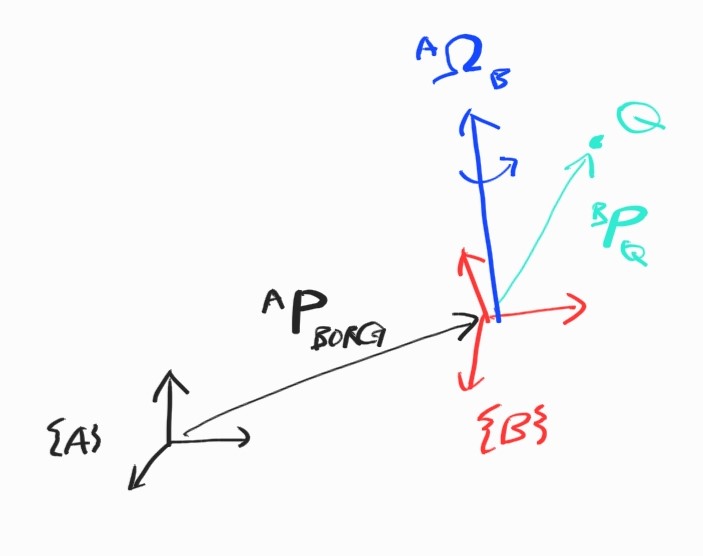
Represented Frame(Reference Frame) 은 물체의 속도를 표현할 때 사용하는 frame이다.
반면 Computed Frame은 속도가 측정되는 frame으로, position이 미분되는 frame을 말한다.
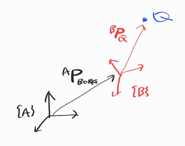
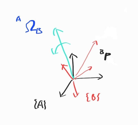
Reference frame을 보다 앞쪽의 superscript로 나타낸다. 예를 들어 $\{B \}$에서 계산되고 $\{A \}$에서 표현되는 velocity vector는
\[{}^{A}({}^{B}\textbf{V}_Q) = \frac{ { }^{A}d}{dt} {}^{B}\textbf{P}_Q\]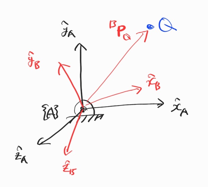
3.2.3 Linear Velocity
점에 기인.
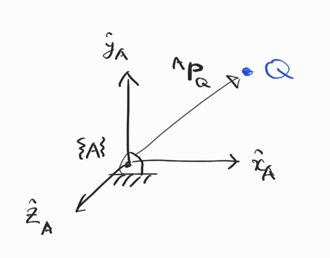
또,
\[{}^{A}\textbf{V}_Q = {}^{A}({}^{A}\textbf{V}_Q) = \frac{ {}^{A}d }{dt} \begin{bmatrix} {}^{A}P_{Qx} \\ {}^{A}P_{Qy} \\ {}^{A}P_{Qz} \\ \end{bmatrix} = \begin{bmatrix} {}^{A}\dot{P}_{Qx} \\ {}^{A}\dot{P}_{Qy} \\ {}^{A}\dot{P}_{Qz} \\ \end{bmatrix}\]Rigid body로 확장하자. Pure translation에서는 ${}^{A} \dot{\textbf{R}}_B = 0$이다.
3.2.4 Angular Velocity
Body에 기인. 한 frame이 다른 frame에 대한 방향의 변화율.
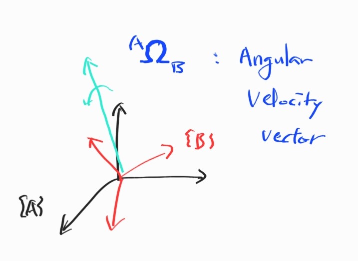
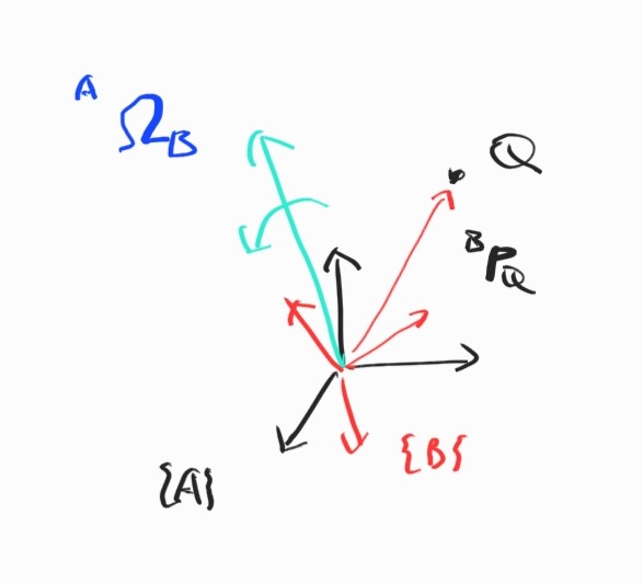
Frame $\{A \}$에 대한 frame $\{B \}$의 회전 변화율은
\[{}^{A} \boldsymbol{\Omega}_B = \begin{bmatrix} \Omega_x \\ \Omega_y \\ \Omega_z \\ \end{bmatrix}\]3.2.5 Rotational Motion of Rigid Body
Rigid body가 각속도 $\boldsymbol{\Omega}$로 회전할 때 강체 위의 점 $P$의 속도 $\textbf{V}_P$는?
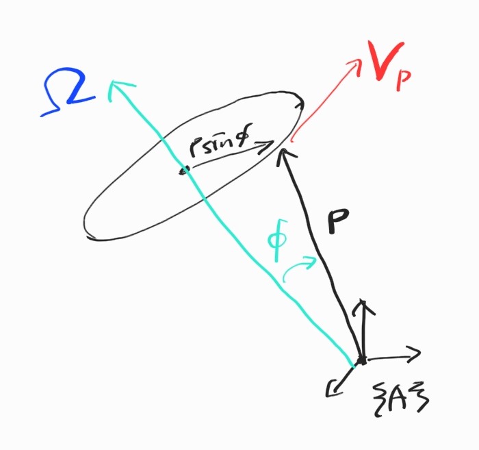
여기서 $\textbf{V}_P$는 $\boldsymbol{\Omega}$와 $\textbf{P}$ 모두에 수직이다. 그러므로,
\[\textbf{V}_P = \boldsymbol{\Omega} \times\textbf{P}\]만약 $Q$가 변화한다면,
OK. 이제 일반적인 식이 구해졌다. linear, angular velocity가 동시에 있을 때,
3.2.6 Derivatives of Orthonormal Matrix
임의의 $n \times n$ orthonormal matrix $\textbf{R}$ 1 에 대해,
\[\textbf{R}\textbf{R}^T = \textbf{I}_n \\ \dot{\textbf{R}}\textbf{R}^T + \textbf{R}\dot{\textbf{R}}^T = \textbf{O}_n \\ \dot{\textbf{R}}\textbf{R}^T + (\dot{\textbf{R}}\textbf{R}^T)^T = \textbf{O}_n\]위 식을 참조하여 새로운 skew-symmetric matrix를 정의할 수 있다.
\[\textbf{S} = \dot{\textbf{R}}\textbf{R}^T \\ \textbf{S} + \textbf{S}^T = \textbf{O}_n\]여기서 우리는 다음 관계식을 얻는다.
\[\dot{\textbf{R}} = \textbf{S}\textbf{R}\]이제 orthonormal matrix의 derivative가 간단해졌다. Skew-symmetric matrix와 곱해주기만 하면 된다.
Skew-symmetric matrix의 특성은 다음과 같다.
\[\textbf{S}^T = -\textbf{S} \textrm{det}(\textbf{S}) = 0\]임의의 matrix는 symmetric matrix와 skew-symmetric matrix의 합으로 표현 가능하다.
또, 임의의 3D 상의 skew-symmetric matrix는 다음과 같이 쓸 수 있다.
\[\textbf{S}(\boldsymbol{\Omega}) = \begin{bmatrix} 0 & -\omega_z & \omega_y \\ \omega_z & 0 & -\omega_x \\ -\omega_y & \omega_x & 0 \end{bmatrix}, \qquad \boldsymbol{\Omega} = \begin{bmatrix} \omega_x \\ \omega_y \\ \omega_z \end{bmatrix}^T\]이제 cross product operator를 사용하면,
\[\textbf{V}_P = \boldsymbol{\Omega} \times \textbf{P} = \textbf{S}\textbf{P}\]3.2.7 Time Derivative of Rotation
$x$-축 방향의 회전을 나타내는 rotation matrix는
\[\textbf{R}_x(\theta) = \begin{bmatrix} 1 & 0 & 0 \\ 0 & \cos \theta & - \sin \theta \\ 0 & \sin \theta & \cos \theta \\ \end{bmatrix}\]이다. 이 행렬을 통해 skew-symmetric matrix를 생성하면
\[\begin{align*} \textbf{S} &= \dot{\textbf{R}}\textbf{R}^T = \frac{d}{d \theta}\textbf{R}_x(\theta) \textbf{R}^T_x(\theta) \\ &= \begin{bmatrix} 0 & 0 & 0 \\ 0 & -\cos \theta & - \cos \theta \\ 0 & \cos \theta & -\sin \theta \\ \end{bmatrix} \begin{bmatrix} 1 & 0 & 0 \\ 0 & \cos \theta & \sin \theta \\ 0 & -\sin \theta & \cos \theta \\ \end{bmatrix} \\ \\ &= \begin{bmatrix} 0 & 0 & 0 \\ 0 & 0 & -1 \\ 0 & 1 & 0 \end{bmatrix} = \textbf{S}(\begin{bmatrix} 1 & 0 & 0 \end{bmatrix}^T) \end{align*}\]그러므로
\[\frac{d}{d \theta}\textbf{R}_x(\theta) = \textbf{S}(\begin{bmatrix} 1 & 0 & 0 \end{bmatrix}^T)\textbf{R}_x(\theta)\]마찬가지로 다른 축에 대해서도 구할 수 있다.
\[\frac{d}{d \theta}\textbf{R}_y(\theta) = \textbf{S}(\begin{bmatrix} 0 & 1 & 0 \end{bmatrix}^T)\textbf{R}_y(\theta) \\ \frac{d}{d \theta}\textbf{R}_z(\theta) = \textbf{S}(\begin{bmatrix} 0 & 0 & 1 \end{bmatrix}^T)\textbf{R}_z(\theta)\]일반적으로,
\[\frac{d}{d \theta}\textbf{R}_k(\theta) = \textbf{S}(\hat{k})\textbf{R}_k(\theta)\]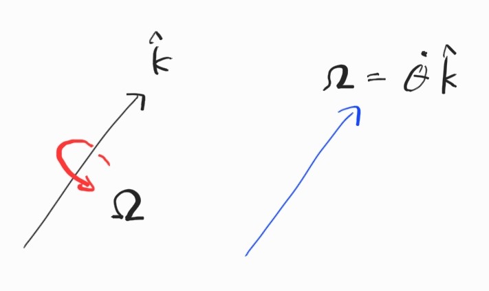
3.2.8 Velocity Due to Rotating Reference Frame
3.2.7 이용.
\[\begin{align*} {}^{A}\textbf{V}_P &= {}^{A}\dot{\textbf{R}}_B {}^{A}\textbf{R}_B^{-1} {}^{A}\textbf{P} \\ &={}^{A}\dot{\textbf{R}}_B {}^{A}\textbf{R}_B^T {}^{A}\textbf{P} \\ &= {}^{A}\textbf{S}_B {}^{A}\textbf{P} = \boldsymbol{\Omega} \times \textbf{P} \end{align*}\]3.2.9 Velocity Propagation
이제야 드디어 Multi-DOF Manipulator의 준비가 되었다. Velocity는 joint를 지나면서 어떻게 전달되는가?
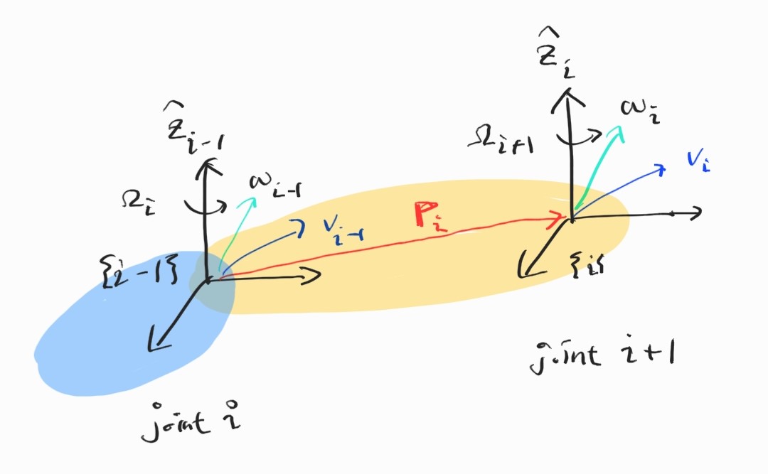
Angular velocity
\[\boldsymbol{\omega}_i = \boldsymbol{\omega}_{i-1} + \boldsymbol{\Omega}_i \\ \boldsymbol{\Omega}_i = \dot{\theta}_i \hat{\textbf{z}}_{i-1}\]Linear velocity
\[\textbf{v}_i = \textbf{v}_{i-1} + \boldsymbol{\omega}_i \times {}^{i-1}\textbf{P}_i + \dot{d}_i \hat{\textbf{z}}_{i-1}\]Revolute joint의 경우라면 $\dot{d}_i=0$일 것이다.
Prismatic joint의 경우는 $\boldsymbol{\Omega}_i=0$.
-
Rotation matrix 등. ↩