
3.1 Differential Kinematics in 2D
3.1.1 Beyond Static Positioning Problem
이제부터는 rigid body의 linear/angular velocity 개념을 사용해 manipulator의 움직임을 분석한다. 또, rigid body에 가해지는 힘을 고려하여 manipulator의 static force에 적용한다.
이 Chapter의 주인공은 다름아닌 Jacobian.
Joint space의 velocity와 Cartesian space의 velocity 사이의 관계는 Jacobian으로 나타난다.
Linear velocity $\textbf{v}$, angular velocity $\boldsymbol{\omega}$를 아울러 spatial velocity $\boldsymbol{\nu}$로 나타내자.
\[\boldsymbol{\nu} = \begin{bmatrix} \textbf{v} \\ \boldsymbol{\omega} \end{bmatrix} = \textbf{J}(\boldsymbol{\theta})\dot{\boldsymbol{\theta}}\]3.1.2 Velocity of 2 DOF Manipulator
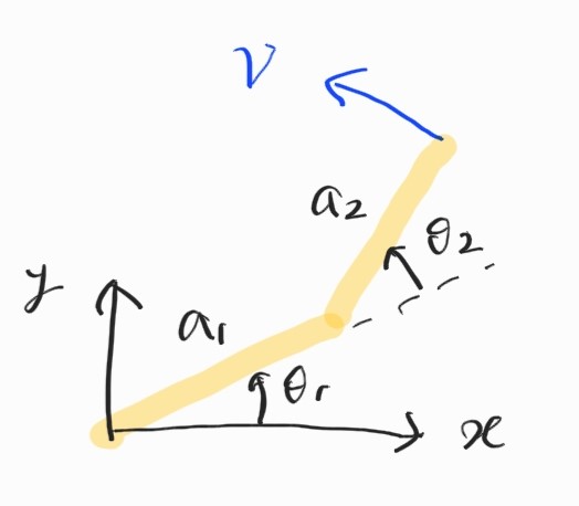
End-effector의 좌표는
\[\xi_E = \begin{bmatrix} x \\ y \end{bmatrix} = \begin{bmatrix} a_1c_1 & a_2c_{12} \\ a_1s_1 & a_2s_{12} \\ \end{bmatrix}\]각 성분에 time derivative를 취하면
\[\dot{x} = -a_1\dot{\theta}_1s_1 - a_2(\dot{\theta}_1+\dot{\theta}_2)s_{12} \\ \dot{y} = a_1\dot{\theta}_1c_1 + a_2(\dot{\theta}_1+\dot{\theta}_2)c_{12} \\\]Matrix form으로는
\[\begin{bmatrix} \dot{x} \\ \dot{y} \end{bmatrix} = \begin{bmatrix} -a_1s_1-a_2s_{12} & -a_2s_{12} \\ a_1c_1+a_2c_{12} & a_2c_{12} \\ \end{bmatrix} \begin{bmatrix} \dot{\theta}_1 \\ \dot{\theta}_2 \end{bmatrix}\]따라서 $\boldsymbol{\nu} = \begin{bmatrix} \textbf{v} \ \boldsymbol{\omega} \end{bmatrix}$과 같은 형태가 완성되고, Jacobian matrix는
\[\textbf{J}(\boldsymbol{\theta}) = \begin{bmatrix} -a_1s_1-a_2s_{12} & -a_2s_{12} \\ a_1c_1+a_2c_{12} & a_2c_{12} \\ \end{bmatrix}\]로 표현된다.
Jacobian의 inverse를 취하자.
\[\dot{\boldsymbol{\theta}} = \textbf{J}(\boldsymbol{\theta})^{-1}\boldsymbol{\nu}\] \[\textbf{J}(\boldsymbol{\theta})^{-1} = \frac{1}{a_2a_2\sin\theta_2} \begin{bmatrix} a_2c_{12} & a_2s_{12} \\ -a_1c_1-a_2c_{12} & -a_1s_1-a_2s_{12} \end{bmatrix}\]Jacobian의 determinant는 $\theta_2=0$이 될 때 $0$이 된다. 이 경우 Jacobian의 inverse는 존재하지 않으며(singularity), manipulator는 하나의 DOF를 잃는다.
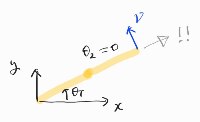
Jacobian determinant가 작으면 특정한 방향으로의 움직임이 매우 어려워진다.
3.1.3 Velocity Ellipse
Unit norm을 가지는 모든 joint velocity들의 set을 생각.
\[\Vert \dot{\boldsymbol{\theta}} \Vert^2 = \dot{\boldsymbol{\theta}} \cdot \dot{\boldsymbol{\theta}} = \dot{\boldsymbol{\theta}}^T\dot{\boldsymbol{\theta}} = 1\]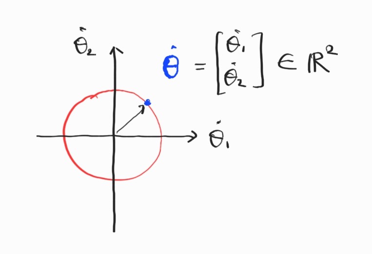
Jacobian inverse를 사용하면,
\[\dot{\boldsymbol{\theta}} = \textbf{J}^{-1} \boldsymbol{\nu} \\ \boldsymbol{\nu}^T(\textbf{J}\textbf{J}^T)\boldsymbol{\nu} = 1\]이 식은 ellipse를 나타내는 방정식이다.
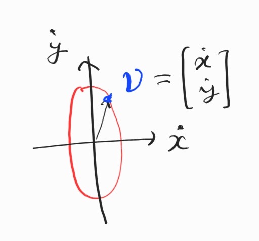
$x$-방향에서 low minimum speed. $y$-방향에서 max high speed.
3.1.4 Velocity of 3 DOF Planar Manipulator
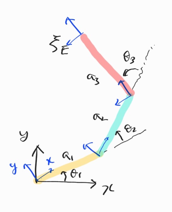
여기까지는 평소대로. Jacobian matrix를 구하자. 미분하고 matrix form으로 바꾸면
\[\begin{bmatrix} \dot{x} \\ \dot{y} \\ \dot{\phi} \end{bmatrix} = \begin{bmatrix} -a_1s_1-a_2s_{12}-a_3s_{123} & -a_2s_{12}-a_3s_{123} & -a_3s_{123} \\ a_1c_1+a_2c_{12}+a_3c_{123} & a_2c_{12}+a_3c_{123} & a_3c_{123} \\ 1 & 1 & 1 \end{bmatrix} \begin{bmatrix} \dot{\theta}_1 \\ \dot{\theta}_2 \\ \dot{\theta}_3 \\ \end{bmatrix}\]이제 Jacobian의 inverse를 구할 수 있다면 주어진 end-effector velocity로부터 joint velocity를 구할 수 있다.
3.1.5 Transforming Spatial Velocity
좌표계 사이에 velocity 변환은 어떻게 이루어질까?
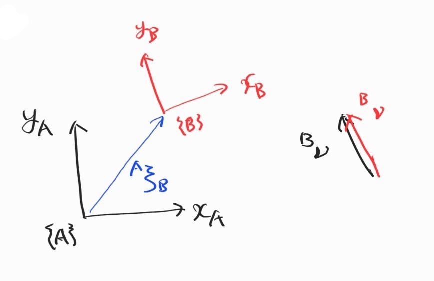
바로 Jacobian.
\[{}^{B}\boldsymbol{\nu} = {}^{B}\textbf{J}_A {}^{A}\boldsymbol{\nu}\] \[{}^{B}\textbf{J}_A = \begin{bmatrix} {}^{B}\textbf{R}_A & \textbf{0}_{2 \times 1} \\ \textbf{0}_{1 \times 2} & 1 \end{bmatrix}\]속도 성분은 rotation matrix에 의해 옮겨지고, 각속도 성분은 그대로.
Velocity Transform of 2 DOF Manipulator
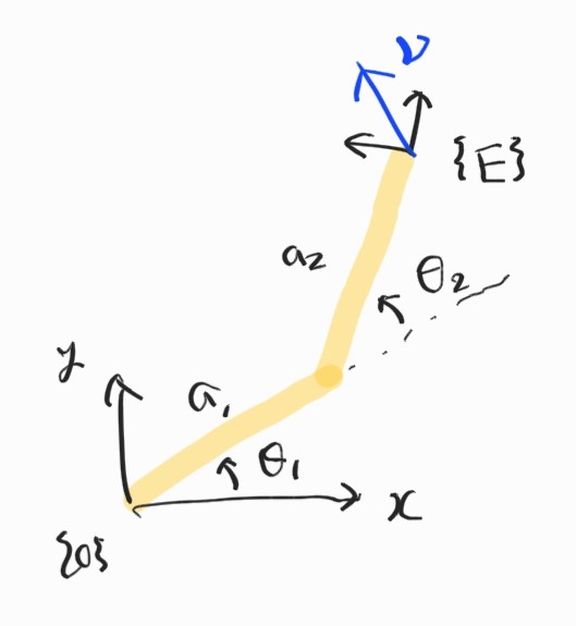
따라서,
\[\begin{align*} {}^{E}\textbf{J}(\boldsymbol{\theta}) &= {}^{E}\textbf{R}_0{}^{0}\textbf{J}(\boldsymbol{\theta}) = \begin{bmatrix} c_12 & s_12 \\ -s_12 & c_12 \end{bmatrix} \begin{bmatrix} -a_1s_1-a_2s_{12} & -a_2s_{12} \\ a_1c_1+a_2c_{12} & a_2c_{12} \\ \end{bmatrix} \\ &= \begin{bmatrix} a_1s_1 & 0 \\ a_1c_2+a_2 & 1 \end{bmatrix} \end{align*}\]