2.4 Inverse Kinematics

---

2.4.1 Inverse Kinematics

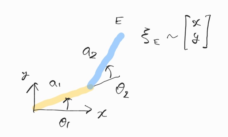
이제부터는 반대로 end-effector pose가 Cartesian space에 주어질 때, 이를 실현시킬 수 있는 $N$개의 joint angle을 찾는 문제를 풀자.

\[\textbf{x} = \begin{bmatrix} x & y & z & \theta_r & \theta_p & \theta_y \end{bmatrix}^T \\ \boldsymbol{\theta} = \begin{bmatrix} \theta_1 & \theta_2 & \theta_3 & \cdots & \theta_N \end{bmatrix}^T\]

Forward kinematics의 경우는 다음과 같은 equation을 풀어야 했다.

\[\textbf{x} = \textbf{K}(\boldsymbol{\theta}) = \textbf{T}_E\]

¹

반대로 inverse kinematics는 $\textbf{T}_E$와 $\textbf{x}$가 주어져 있을 때,

\[\boldsymbol{\theta} = \textbf{K}^{-1}(\textbf{x}) \in \mathbb{R}^N\]

를 구하는 문제가 된다.

다시 말해, homogeneous transform이 주어져 있다.

\[\textbf{T}_E = \begin{bmatrix} \textbf{R}_E & \textbf{p}_E \\ 0 & 1 \end{bmatrix}\]

이제 다음을 만족하는 해 $\theta_1, \theta_2, \cdots, \theta_N$을 찾아라!

\[\textbf{T}_E = {}^{0}\textbf{T}_1(\theta_1){}^{1}\textbf{T}_2(\theta_2) \cdots {}^{N-1}\textbf{T}_N(\theta_N){}^{N}\textbf{T}_E(\bullet)\]

Method of Solutions

Inverse kinematics를 해결하는 일반적인 방법은 없다.

  (1) Closed form solution : algebraic expression과 같은 non-iterative solution.

• Geometric
• algebraic

  (2) Numerical solution : iterative, numerical.

• 계산에 많은 노력이 필요하고 오래 걸린다.

---

2.4.1 2 DOF Planar Manipulator

Geometric Approach

\[\xi_E = \begin{bmatrix} x \\ y \end{bmatrix} = \begin{bmatrix} a_1c_1 + a2c_{12} \\ a_1s_1 + a2s_{12} \end{bmatrix}\] \[r^2 = x^2 + y^2\]

먼저 해의 존재성을 생각하자.

Worskpace란 간단히 말해서 manipulator의 end-effector가 도달할 수 있는 space의 volume을 의미한다.

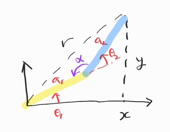
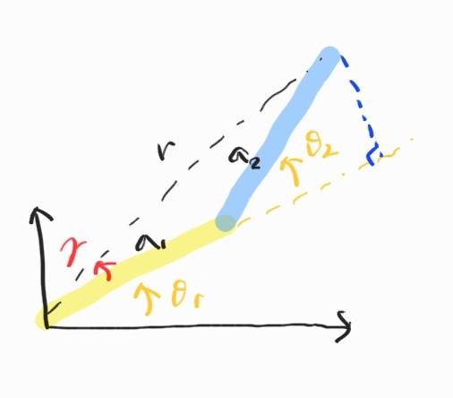
위 그림에 해당하는 위치에 end-effector가 도달할 수 있으려면, 즉 해가 존재하려면 다음 식을 만족해야 한다.

\[(a_1 - a_2)^2 \leq x^2 + y^2 \leq (a_1 + a_2)^2 \\ \\ \textrm{or} \\ \\ \vert a_1 - a_2 \vert \leq \Vert \textbf{P}_E \Vert \leq a_1 + a_2\]

여기서 $\textbf{P}_E = \begin{bmatrix} x & y \end{bmatrix}^T$.

이제 기하학적인 지식을 동원해 해를 구하자. 먼저 제2코사인법칙.

\[\begin{align*} r^2 &= x^2 + y^2 \\ &= a_1^2 + a_2^2 - 2a_1a_2 \cos \alpha \end{align*}\]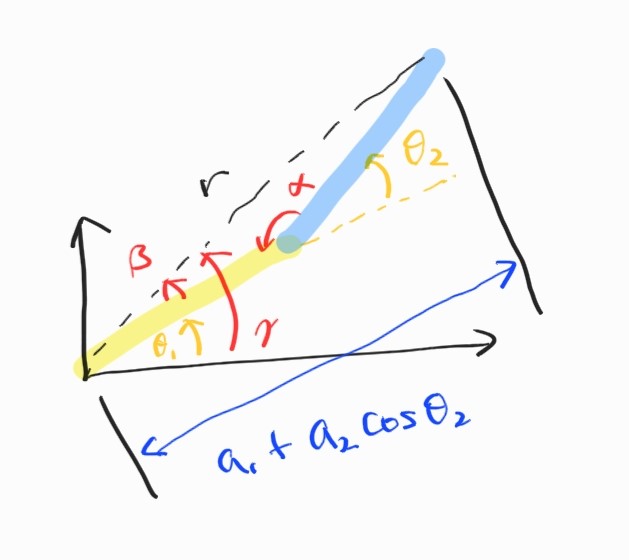

\[\begin{align*} \cos \alpha &= \frac{a_1^2 + a_2^2 - r^2}{2a_1a_2} \\ \\ &= \frac{a_1^2 + a_2^2 - x^2 - y^2}{2a_1a_2} \end{align*}\]

\[\begin{align*} \theta_2 &= \pi - \alpha \\ \cos \theta_2 &= - \cos \alpha \end{align*}\]

\[\sin \theta_2 = \sqrt{1 - \cos \theta_2^2}\] \[\beta = \tan^{-1} \frac{a_2 \sin \theta_2}{a_1 + a^@ \cos \theta_2}\] \[\gamma = \tan^{-1} \frac{y}{x}\] \[\theta_1 = \gamma - \beta = \tan^{-1} \frac{y}{x} - \tan^{-1} \frac{a_2 \sin \theta_2}{a_1 + a^2 \cos \theta_2}\] \[\theta_2 = \cos^{-1}\frac{a_1^2 + a_2^2 - x^2 - y^2}{2a_1a_2}\]

이것으로 두 joint angle을 모두 구할 수 있었다.

그런데, 한 가지 해가 더 존재한다. elbow가 위쪽에 있을 경우.

\[\theta_2 = -\cos^{-1}\frac{x^2 + y^2 - a_1^2 - a_2^2}{2a_1a_2}\] \[\gamma = \tan^{-1} \frac{y}{x}\] \[\theta_1 = \gamma + \beta = \tan^{-1} \frac{y}{x} + \tan^{-1} \frac{a_2 \sin \theta_2}{a_1 + a^2 \cos \theta_2}\]

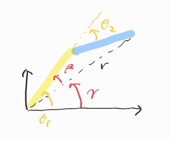
그러므로 2개의 해가 존재한다.

Algebraic Approach

Homogeneous matrix를 계산하면,

\[\textbf{T}_E = \begin{bmatrix} \cos(\theta_1 + \theta_2) & -\sin(\theta_1 + \theta_2) & a_1 \cos \theta_1 + a_2 \cos (\theta_1 + \theta_2) \\ \sin(\theta_1 + \theta_2) & \cos(\theta_1 + \theta_2) & a_1 \sin \theta_1 + a_2 \sin (\theta_1 + \theta_2) \\ 0 & 0 & 1 \end{bmatrix}\]

그러므로,

\[x = a_1 \cos \theta_1 + a_2 \cos (\theta_1 + \theta_2) = (a_1 + a_2c_2)c_1 - a_2s_2s_1 \\ y = a_1 \sin \theta_1 + a_2 \sin (\theta_1 + \theta_2) = (a_1 + a_2c_2)s_1 + a_2s_2c_1\]

풀기 쉽게 정리하자.

\[x = k_1 c_1 - k_2 s_1 \\ y = k_1 s_1 + k_2 c_1 \\ k_1 = a_1 + a_2c_2 \\ k_2 = a_2s_2\] \[k_1 = r \cos \gamma \\ k_2 = r \sin \gamma \\\] \[\frac{x}{r} = \cos \gamma \cos \theta_1 - \sin \gamma \sin \theta_1 \\ \frac{y}{r} = \cos \gamma \sin \theta_1 + \sin \gamma \cos \theta_1\]

이제 joint angle을 구하면

\[\cos (\gamma + \theta_1) = \frac{x}{r} \\ \sin (\gamma + \theta_1) = \frac{y}{r}\] \[\gamma + \theta_1 = \tan^{-1} \frac{y}{x}\] \[\theta_1 = \tan^{-1}\frac{y}{x} - \tan^{-1}\frac{a_2s_2}{a_1+a_2c_2}\]

$\theta_2$는 제2코사인법칙으로.

---

2.4.2 Solvability

모든 solution들의 set이 결정될 수 있다면, manipulator가 solvable하다고 한다.

Kinematics의 중요한 결과 중 하나는, revolute joint와 prismatic joint가 하나의 chain으로 이루어진 6 DOF system은 모두 solvable하다는 것.

다만 그 해는 numerical. 6 DOF manipulator 중에서도 특별한 case들만이 analytic하게 풀 수 있다.

Analytic solution을 구하는 방법을 요약하면 다음과 같다.

  (1) DH paremeter를 이용해 로봇을 modeling.

  (2) Forward kinematic equation을 작성.

  (3) 12개 equation으로부터 unknown joint variable을 유도한다.

  (4) Multiple configuration을 다룬다.

---

2.4.3 Pieper’s Solution

Pieper는 6 DOF manipulator 중에서 세 연속된 축이 한 점에서 교차하는 경우를 연구했다. 여기서는 마지막 세 revolute joint가 교차하는 case를 알아본다.

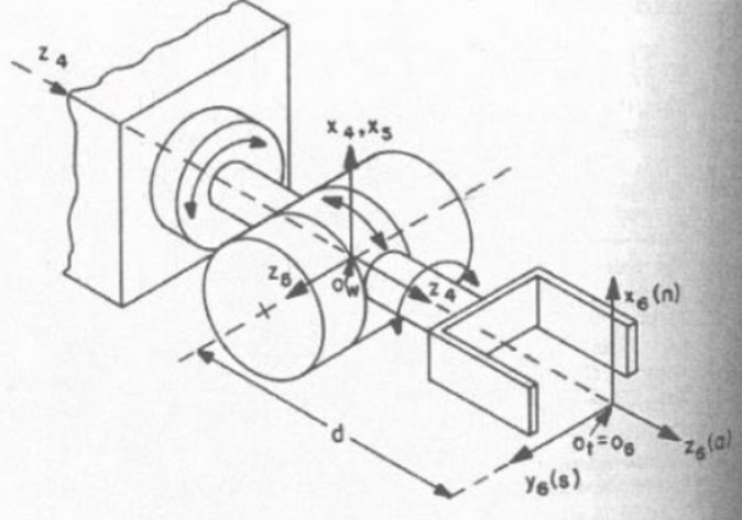
Link frame $\{4 \}$, $\{5 \}$, $\{6 \}$이 한 점에서 교차한다고 하자. 이 점은 base coordinate에서

\[{}^{0}\textbf{P}_{4ORG} = {}^{0}\textbf{T}_1{}^{1}\textbf{T}_2{}^{2}\textbf{T}_3{}^{3}\textbf{P}_{4ORG} = \begin{bmatrix} x \\ y \\ z \\ 1 \end{bmatrix}\]

로 표현된다. ${}^{i-1}\textbf{T}_i$의 일반적인 형태를 떠올려보자. 2.2.3의 Craig’s convention을 따르면,

\[{}^{0}\textbf{P}_{4ORG} = {}^{0}\textbf{T}_1{}^{1}\textbf{T}_2{}^{2}\textbf{T}_3 \begin{bmatrix} a_3 \\ -d_4 \sin \alpha_3 \\ d_4 \cos \alpha_3 \\ 1 \end{bmatrix}\]

또는,

\[{}^{0}\textbf{P}_{4ORG} = {}^{0}\textbf{T}_1{}^{1}\textbf{T}_2 \begin{bmatrix} f_1(\theta_3) \\ f_2(\theta_3) \\ f_3(\theta_3) \\ 1 \end{bmatrix}, \qquad \begin{bmatrix} f_1 \\ f_2 \\ f_3 \\ 1 \end{bmatrix} = {}^{2}\textbf{T}_3 \begin{bmatrix} a_3 \\ -d_4 s \alpha_3 \\ d_4 c \alpha_3 \\ 1 \end{bmatrix}\]

${}^{2}\textbf{T}_3$ 역시 DH parameter로 계산 가능하므로,

\[\begin{align*} f_1 &= a_3c_3 + d_4s\alpha_3s_3 + a_2 \\ f_2 &= a_3c\alpha_2s_3 - d_4s\alpha_3c\alpha_2c_3 - d_4s\alpha_2c\alpha_3 - d_3s\alpha_2 \\ f_3 &= a_3s\alpha_2s_3 - d_4s\alpha_3s\alpha_2c_3 + d_4c\alpha_2c\alpha_3 + d_3c\alpha_2 \\ \end{align*}\]

마찬가지로 ${}^{0}\textbf{T}_1$, ${}^{0}\textbf{T}_2$를 계산하고…

\[{}^{0}\textbf{P}_{4ORG} = \begin{bmatrix} c_1g_1-s_1g_2 \\ s_1g_1+c_1g_2 \\ g_3 \\ 1 \end{bmatrix}\] \[\begin{align*} g_1 &= c_2f_1 - s_2f_2 + a_1 \\ g_2 &= s_2c\alpha_1f_1 + c_2c\alpha_1f_2 - s\alpha_1f_3 - d_2s\alpha_1 \\ g_3 &= s_2s\alpha_1f_1 + c_2s\alpha_1f_2 + c\alpha_1f_3 + d_2c\alpha_1 \\ \end{align*}\]

이제 ${}^{0}\textbf{P}_{4ORG}$의 크기 제곱을 $r=x^2+y^2+z^2$라고 하면 위 식에 의해,

\[r=g_1^2+g_2^2+g_3^2\]

이고,

\[r=f_1^2+f_2^2+f_3^2 + a_1^2+d_2^2+2d_2f_3 + 2a_1(c_2f_1 - s_2f_2)\]

이 식에는 더이상 $\theta_1$가 남아있지 않다.

---

2.4.4 Inverse Kinematics for PUMA 560

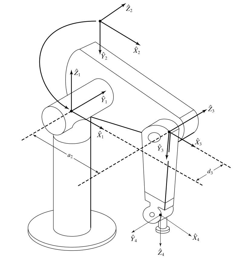
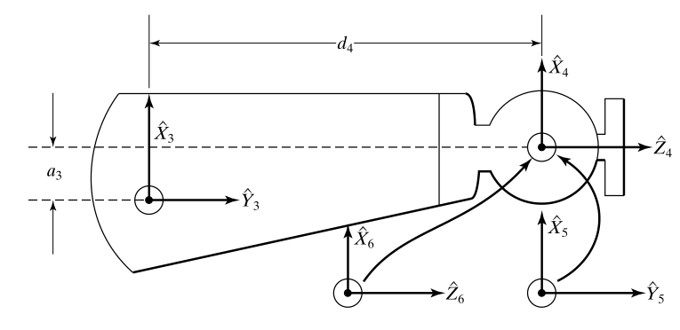
6개의 revolute joint를 갖는 puma 560 로봇. 마지막 세 joint는 한 점에서 만난다.

DH parameter는 Craig’s convention을 사용했다.

$i$	$\alpha_{i-1}$	$a_{i-1}$	$d_u$	$\theta_j$
1	0	0	0	$\theta_1$
2	-90	0	0	$\theta_2$
3	0	$a_2$	$d_3$	$\theta_3$
4	-90	$a_3$	$d_4$	$\theta_4$
5	90	0	0	$\theta_5$
6	90	0	0	$\theta_6$

Transformation matrix 계산은 여차저차…

  (1) Tool position ${}^{0}\textbf{T}_6$를 구한다. DH parameter를 사용.

  (2) Forward kinematics ${}^{0}\textbf{T}_6(\theta_1, \theta_2, \theta_3)$와 rotation kinematics ${}^{3}\textbf{R}_6(\theta_4, \theta_5, \theta_6)$을 푼다.

  (3) ${}^{0}\textbf{T}_6$의 마지막 column으로부터 wrist center의 위치 $\textbf{P}_c$를 찾는다.

  (4) $\textbf{P}_c$는 ${}^{0}\textbf{T}_3(\theta_1, \theta_2, \theta_3)$의 마지막 column이기도 하므로 이로부터 $\theta_1, \theta_2, \theta_3$를 구한다.

  (5) $\theta_1, \theta_2, \theta_3$를 대입하여 ${}^{3}\textbf{R}_6 = {}^{0}\textbf{R}_3^{-1}{}^{0}\textbf{R}_6$를 구한다.

  (6) ${}^{3}\textbf{R}_6 = {}^{3}\textbf{R}_6(\theta_4, \theta_5, \theta_6)$이므로 이로부터 $\theta_4, \theta_5, \theta_6$를 구한다.

Step 1

3D space 상에서 wrist의 pose가 주어져 있다고 하자.

\[\begin{align*} {}^{0}\textbf{T}_6 &= {}^{0}\textbf{T}_1{}^{1}\textbf{T}_2{}^{2}\textbf{T}_3{}^{3}\textbf{T}_4{}^{4}\textbf{T}_5{}^{5}\textbf{T}_6 \\ \\ &= \begin{bmatrix} \textbf{R} & \textbf{p} \\ 0 & 1 \\ \end{bmatrix} = \begin{bmatrix} r_{11} & r_{12} & r_{13} & p_x \\ r_{21} & r_{22} & r_{23} & p_y \\ r_{31} & r_{32} & r_{33} & p_z \\ 0 & 0 & 0 & 1 \end{bmatrix} \end{align*}\]

Step 2

Wrist pose의 함수로써 표현되는 joint angle을 찾자.

\[\textbf{x} = \begin{bmatrix} p_x & p_y & p_z & \alpha & \beta & \gamma \end{bmatrix}^T\] \[\textbf{x} = f(\boldsymbol{\theta}) = {}^{0}\textbf{T}_N\] \[\boldsymbol{\theta} = f^{-1}(\textbf{x})\]

Step 3

Kinematics equation의 양변에 transformation matrix의 inverse를 곱하여 찾고자 하는 변수를 분리해낸다.

\[[{}^{0}\textbf{T}_1(\theta_1)]^{-1}{}^{0}\textbf{T}_6 = [{}^{0}\textbf{T}_1(\theta_1)]^{-1}{}^{0}\textbf{T}_1{}^{1}\textbf{T}_2{}^{2}\textbf{T}_3{}^{3}\textbf{T}_4{}^{4}\textbf{T}_5{}^{5}\textbf{T}_6\]

예를 들면 좌변의 $[{}^{0}\textbf{T}_1(\theta_1)]^{-1}$는 $\theta_1$에 대한 함수이며 ${}^{0}\textbf{T}_6$는 주어져 있다. 여기서 $\theta_1$과 $\theta_3$를 분리하여 계산할 수 있다.

\[[{}^{0}\textbf{T}_3(\theta_1, \theta_2, \theta_3)]^{-1}{}^{0}\textbf{T}_6 = [{}^{0}\textbf{T}_3(\theta_1, \theta_2, \theta_3)]^{-1}{}^{0}\textbf{T}_1{}^{1}\textbf{T}_2{}^{2}\textbf{T}_3{}^{3}\textbf{T}_4{}^{4}\textbf{T}_5{}^{5}\textbf{T}_6\]

그 다음은 $\theta_2$와 $\theta_4$를 따로 계산. 마지막으로,

\[[{}^{0}\textbf{T}_4(\theta_1, \theta_2, \theta_3, \theta_4)]^{-1}{}^{0}\textbf{T}_6 = [{}^{0}\textbf{T}_4(\theta_1, \theta_2, \theta_3, \theta_4)]^{-1}{}^{0}\textbf{T}_1{}^{1}\textbf{T}_2{}^{2}\textbf{T}_3{}^{3}\textbf{T}_4{}^{4}\textbf{T}_5{}^{5}\textbf{T}_6\] \[[{}^{0}\textbf{T}_5(\theta_1, \theta_2, \theta_3, \theta_4, \theta_5)]^{-1}{}^{0}\textbf{T}_6 = [{}^{0}\textbf{T}_5(\theta_1, \theta_2, \theta_3, \theta_4, \theta_5)]^{-1}{}^{0}\textbf{T}_1{}^{1}\textbf{T}_2{}^{2}\textbf{T}_3{}^{3}\textbf{T}_4{}^{4}\textbf{T}_5{}^{5}\textbf{T}_6\]

이렇게 $\theta_5$와 $\theta_6$까지 계산하면 끝. 여기까지가 전체적인 계산 절차이다.

Step 4

${}^{0}\textbf{T}_1$의 inverse를 구하는 것은 간단하다.

\[[{}^{A}\textbf{T}_B(\theta_1)]^{-1} = {}^{B}\textbf{T}_A = \begin{bmatrix} {}^{A}\textbf{R}_B^T & -{}^{A}\textbf{R}_B^T {}^{A}\textbf{P}_{BORG} \\ \textbf{0} & 1 \end{bmatrix}\]

이므로,

\[{}^{0}\textbf{T}_1 = \begin{bmatrix} c_1 & -s_1 & 0 & 0 \\ s_1 & c_1 & 0 & 0 \\ 0 & 0 & 1 & 0 \\ 0 & 0 & 0 & 1 \end{bmatrix} \qquad [{}^{0}\textbf{T}_1]^{-1} = \begin{bmatrix} c_1 & s_1 & 0 & 0 \\ -s_1 & c_1 & 0 & 0 \\ 0 & 0 & 1 & 0 \\ 0 & 0 & 0 & 1 \end{bmatrix}\]

이 행렬을 양변에 곱하게 되면,

\[\begin{bmatrix} c_1 & s_1 & 0 & 0 \\ -s_1 & c_1 & 0 & 0 \\ 0 & 0 & 1 & 0 \\ 0 & 0 & 0 & 1 \end{bmatrix} \begin{bmatrix} r_{11} & r_{12} & r_{13} & p_x \\ r_{21} & r_{22} & r_{23} & p_y \\ r_{31} & r_{32} & r_{33} & p_z \\ 0 & 0 & 0 & 1 \end{bmatrix} = {}^{1}\textbf{T}_6\]

Step 5

위 식을 계산해야 한다. 먼저 DH parameter로 얻은 transformation matrix를 어찌저찌 계산하면…

\[{}^{1}\textbf{T}_6 = \begin{bmatrix} {}^{1}r_{11} & {}^{1}r_{12} & {}^{1}r_{13} & {}^{1}p_x \\ {}^{1}r_{21} & {}^{1}r_{22} & {}^{1}r_{23} & {}^{1}p_y \\ {}^{1}r_{31} & {}^{1}r_{32} & {}^{1}r_{33} & {}^{1}p_z \\ 0 & 0 & 0 & 1 \end{bmatrix}\] \[\begin{align*} {}^{1}r_{11} &= c_{23}[c_4c_5c_6-s_4s_6]-s{23}s_5s_6 \\ {}^{1}r_{21} &= -s_4c_5c_6-c_4s_6 \\ {}^{1}r_{31} &= -s_{23}[c_4c_5c_6-s_4s_6]-c{23}s_5c_6 \\ {}^{1}r_{12} &= -c_{23}[c_4c_5s_6+s_4c_6]+s{23}s_5s_6 \\ {}^{1}r_{22} &= s_4c_5s_6-c_4c_6 \\ {}^{1}r_{32} &= s_{23}[c_4c_5s_6+s_4c_6]+c{23}s_5s_6 \\ {}^{1}r_{13} &= -c_{23}c_4s_5 - c_{23}c_5 \\ {}^{1}r_{23} &= s_4s_5 \\ {}^{1}r_{33} &= s_{23}c_4s_5 - c_{23}c_5 \\ {}^{1}p_x &= a_2c_2 + a_3c_{23}-d_4s_{23} \\ {}^{1}p_y &= d_3 \\ {}^{1}p_z &= -a_3s_{23} -a_2s_2 - d_4c_{23} \end{align*}\]

휴.

$(2,4)$ 성분을 계산하자. 즉 첫 번째 행렬의 2행과 두 번째 행렬의 4열을 곱하면,

\[-s_1p_x + c_1p_y = d_3\]

Trigonometric substitution을 통해,

\[p_x = \rho \cos \phi \\ p_x = \rho \sin \phi \\ \phi = \textrm{atan2}(p_y, p_x)\] \[c_1s_{\phi} - s_1c_{\phi} = \frac{d_3}{\rho} \\ \sin(\phi - \theta_1) = \frac{d_3}{\rho}\] \[\cos(\phi - \theta_1) = \pm \sqrt{1-\left( \frac{d_3}{\rho}\right)^2} \\ \phi - \theta_1 = \textrm{atan2}\left( \frac{d_3}{\rho}, \pm \sqrt{1-\left( \frac{d_3}{\rho}\right)^2} \right)\]

따라서 $\theta_1$을 구할 수 있게 되었다.

\[\theta_1 = \textrm{atan2}(p_y, p_x) - \textrm{atan2}\left( \frac{d_3}{\rho}, \pm \sqrt{1-\left( \frac{d_3}{\rho}\right)^2} \right)\]

이를 만족하는 해는 2개.

---

Step 6~

자, 이런 식으로 다른 성분들도 계산하고… 아무튼 해를 구할 수 있으니 생략. 사람이 할 일이 아니다.

---

1. 여기서 $\textbf{T}_E$는 12개 equation. ↩