
2.1 Forward Kinematics
Kinematics란 body 또는 이들의 system의 운동을 연구하는 학문. 이때 질량이나 가해지는 힘은 생각하지 않는다.
Robot arm(manipualtor)은 rigid link들과 joint들의 chain으로 이루어져 있다. 각 joint는 1 DOF를 가지며 translational(sliding/prismatic joint)하고나 rotational(revolute joint)하다.
Chain의 한쪽 끝(base)는 일반적으로 고벙되어 있으며 반대쪽 끝(end-effector)은 공간 상에서 자유롭게 움직인다.
Forward Kinematics란 joint coordinat 또는 robot configuration으로부터 end-effector pose로의 mapping.
먼저 가장 단순한 것부터 시작하자.
2.1.1 1 DOF Planar Manipulator
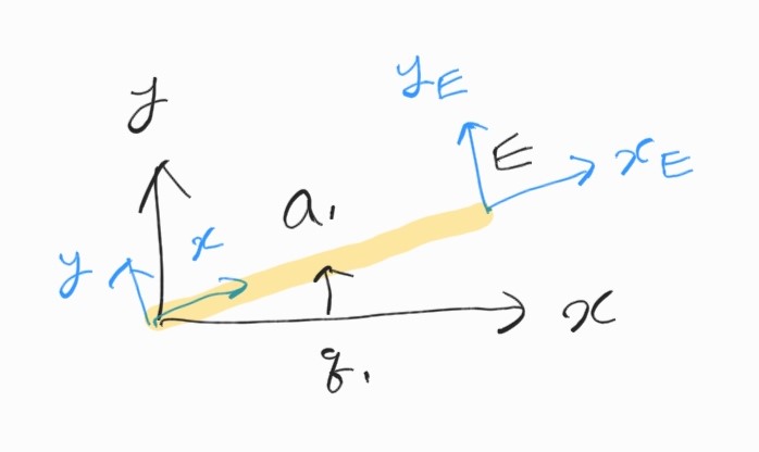
하나의 Link가 땅에 고정되어 있다고 하자. 연결된 joint에는 모터가 장착되어 있어서 회전이 가능하다. $\{0 \}$ frame과 end effector $\{E \}$ frame 사이의 관계는?
Link의 길이를 $a_1$, 각도를 $q_1$이라고 하면 $\{0 \}$에서 본 end-effector의 좌표는 다음과 같다.
\[\begin{bmatrix} x \\ y \end{bmatrix} = \begin{bmatrix} a_1 \cos q_1 \\ a_1 \sin q_1 \\ \end{bmatrix}\]보다 일반적으로 두 frame 사이의 관계를 구하기 위해,
\[\xi_{E} = \mathbf{T}_{E} = \mathbf{R}(q_1)\mathbf{T}_x(a_1)\]즉 $\{E \}$는 $\{0 \}$을 각도 $q_1$만큼 rotate, 길이 $a_1$만큼 traslate시킨 것.
Transformation matrix를 사용해 간단히 계산할 수 있다.
\[\begin{align*} \mathbf{T}_E &= \begin{bmatrix} \cos q_1 & -\sin q_1 & 0 \\ \sin q_1 & \cos q_1 & 0 \\ 0 & 0 & 1 \end{bmatrix} \begin{bmatrix} 1 & 0 & a_1 \\ 0 & 1 & 0 \\ 0 & 0 & 1 \end{bmatrix} \\ \\ &= \begin{bmatrix} \cos q_1 & -\sin q_1 & a_1 \cos q_1 \\ \sin q_1 & \cos q_1 & a_1 \sin q_1 \\ 0 & 0 & 1 \end{bmatrix} \end{align*}\]Robotics Toolbox - 1 DOF Manipulator
trchain2(s, q) 함수는 string s에 해당하는 homogeneous transform($3 \times 3$)을 반환한다. 이때 사용되는 각도 변수의 이름은 column vector q의 성분이다.
a1 = 1;
q1 = 0.2;
trchain2('R(q1) Tx(a1)', q1)

---

ans =

    0.9801   -0.1987    0.9801
    0.1987    0.9801    0.1987
         0         0    1.0000
위 코드는 다음을 계산한 것과 같다.
trot(0.2) * transl2(1, 0)
q1과 a1을 symbolic 처리한 다음에 결과를 보자.
syms q1 a1;
trchain2('R(q1) Tx(a1)', q1)

---

ans =

[cos(q1), -sin(q1), a1*cos(q1)]
[sin(q1),  cos(q1), a1*sin(q1)]
[      0,        0,          1]
간단한 model을 생성해 보자.
% create the workspace variable p1
% which describes the kinematic characteristics of a simple planar 1-link mechanism.
mdl_planar1

% drive the graphical robot
p1.teach
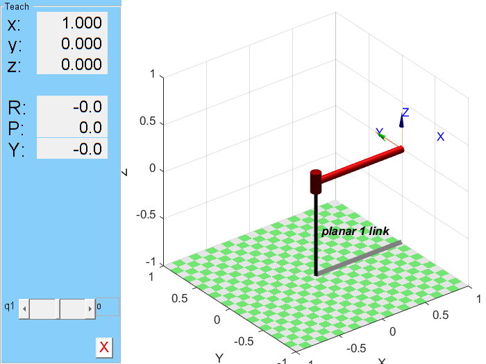
q1을 조절해가며 manipulator의 움직임을 확인할 수 있다.
2.1.2 2 DOF Planar Manipulator
2개의 link와 2개의 revolute joint를 갖는 planar manipulator. 이 경우 역시 두 joint에 모터가 달려있는 것처럼 생각하자.
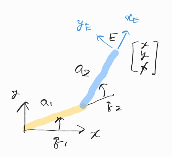
같은 방법으로,
\[\begin{bmatrix} x \\ y \end{bmatrix} = \begin{bmatrix} a_1c_1+a_2c_{12} \\ a_1s_1+a_2s_{12} \\ \end{bmatrix}\] \[\begin{align*} \mathbf{T}_E &= \mathbf{R}(q_1) \mathbf{T}_x(a_1) \mathbf{R}(q_2) \mathbf{T}_x(a_2) \\ \\ &= \begin{bmatrix} c_{12} & -s_{12} & a_1c_1+a_2c_{12} \\ s_{12} & c_{12} & a_1s_1+a_2s_{12}\\ 0 & 0 & 1 \end{bmatrix} \end{align*}\]여기서 2D transform이므로 $\mathbf{T}_E = SE(2)$
Robotics Toolbox - 2 DOF Manipulator
syms q1 q2 a1 a2;
trchain2('R(q1) Tx(a1) R(q2) Tx(a2)', [q1 q2])
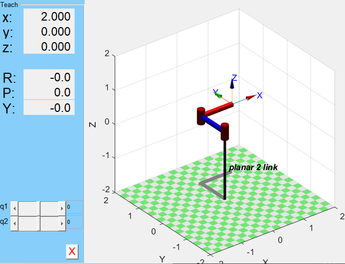
mdl_planar2;
p2.teach
---
ans =
[cos(q1)*cos(q2) - sin(q1)*sin(q2), - cos(q1)*sin(q2) - cos(q2)*sin(q1), a2*(cos(q1)*cos(q2) - sin(q1)*sin(q2)) + a1*cos(q1)]
[cos(q1)*sin(q2) + cos(q2)*sin(q1), cos(q1)*cos(q2) - sin(q1)*sin(q2), a2*(cos(q1)*sin(q2) + cos(q2)*sin(q1)) + a1*sin(q1)]
[ 0, 0, 1]

q1, q2값을 지정했을 때의 결과를 보고 싶다면 plot 명령어를 사용한다.
p2.plot([pi/2, -pi/2])
이제 유사한 방식으로 3 DOF도…
-
여기서 $\mathbf{T}_{E} = {}^{0}\mathbf{T}_{E}$. ↩