
1.2 Working in 2D
2D 세상, plane에서는 익숙한 Euclidean geometry가 있다. Cartesian coord. frame은 수평축 $x$-축과 수직축 $y$-축으로 이루어진다. 두 축의 교점을 origin이라고 한다.
두 축에 평행한 단위 벡터들을 $\hat{\textbf{x}}$, $\hat{\textbf{y}}$로 나타내자. 이 $x$-, $y$-축에 대한 point의 좌표는 $(x,y])$ 또는 벡터
\[p=x \hat{\textbf{x}} + y \hat{\textbf{y}} \tag{ $1$ }\]로 표현된다.
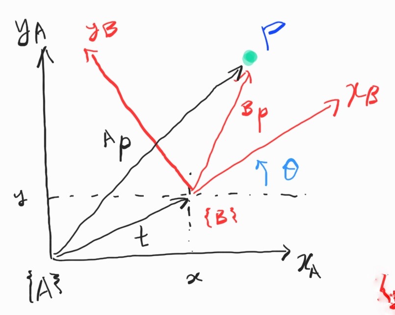
$\{B\}$의 원점이 $\{A\}$에 대해 어디에 위치해 있는지 보자. 벡터 $\textbf{t}=\begin{bmatrix}x&y\end{bmatrix}$만큼 떨어져 있으며, 반시계 방향으로 각도 $\theta$만큼 회전해 있다.
따라서, pose를 표현하는 구체적인 기호는 3-vector $^{A}\xi_{B}\sim \begin{bmatrix}x&y&\theta\end{bmatrix}$이다.1
그치만 아쉽게도 이 표현식은 그리 편리하지는 않다. 예를 들어 composition
\[\begin{bmatrix}x_{1}&y_{1}&\theta_{1}\end{bmatrix} \oplus \begin{bmatrix}x_{2}&y_{2}&\theta_{2}\end{bmatrix}\]은 두 pose의 복잡한 삼각 함수로 이루어져 있다. 둘로 나누어서 고려하자. rotation과 translation.
1.2.1 Orientation in 2D
Orthonormal Rotation matrix
새로운 frame $\{V\}$를 생각하자. Frame $\{V\}$는 $\{A\}$와 평행하면서 원점이 $\{B\}$와 같은 frame이다.
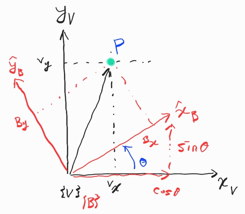
식 $(1)$에 의하면 $\{V\}$에 대한 점 $\textbf{P}$는 frame의 축에서 정의된 단위벡터들을 이용해,
\[\begin{align*} {}^{V}\textbf{p} &= {}^{V}x\hat{\textbf{x}}_V + {}^{V}y\hat{\textbf{y}}_V \\ &= \begin{bmatrix} \hat{\textbf{x}}_V & \hat{\textbf{y}}_V \end{bmatrix} \begin{bmatrix} {}^{V}x \\ {}^{V}y \end{bmatrix} \\ \end{align*} \tag{ $ 2 $ }\]이렇게 row vector와 column vector의 곱으로 표현된다.
coord. frame $\{B \}$ 역시 이 수직인 두 단위 벡터들로 표현할 수 있다.
\[\begin{align*} \hat{\textbf{x}}_B &= \cos \theta \hat{\textbf{x}}_V + \sin \theta \hat{\textbf{y}}_V \\ \hat{\textbf{y}}_B &= -\sin \theta \hat{\textbf{x}}_V + \cos \theta \hat{\textbf{y}}_V \\ \end{align*}\]역시 행렬 표현으로,
\[\begin{bmatrix} \hat{\textbf{x}}_B & \hat{\textbf{y}}_B \end{bmatrix} = \begin{bmatrix} \hat{\textbf{x}}_V & \hat{\textbf{y}}_V \end{bmatrix} \begin{bmatrix} \cos \theta & -\sin \theta \\ \sin \theta & \cos \theta \\ \end{bmatrix} \tag{ $3$ }\]다시 식 $(1)$를 이용하면 $\{B \}$에 대한 point $\textbf{P}$는
\[\begin{align*} {}^{B}\textbf{p} &= {}^{B}x\hat{\textbf{x}}_B + {}^{B}y\hat{\textbf{y}}_B \\ &= \begin{bmatrix} \hat{\textbf{x}}_B & \hat{\textbf{y}}_B \end{bmatrix} \begin{bmatrix} {}^{B}x \\ {}^{B}y \end{bmatrix} \\ \end{align*}\]여기에 식 $(3)$를 적용하면,
\[\begin{align*} {}^{B}\textbf{p} = \begin{bmatrix} \hat{\textbf{x}}_V & \hat{\textbf{y}}_V \end{bmatrix} \begin{bmatrix} \cos \theta & -\sin \theta \\ \sin \theta & \cos \theta \\ \end{bmatrix} \begin{bmatrix} {}^{B}x \\ {}^{B}y \end{bmatrix} \end{align*} \tag{ $ 4 $ }\]식 $(2)$와 $(4)$을 보자. 두 식의 우변은 모두 단위벡터 $\hat{\textbf{x}}_V$, $\hat{\textbf{y}}_V$로 표현되어 있다. 둘은 같은 점 $\textbf{P}$를 나타낸 것이므로 계수를 같게 둘 수 있다. 즉,
\[\begin{bmatrix} {}^{V}x \\ {}^{V}y \end{bmatrix} = \begin{bmatrix} \cos \theta & -\sin \theta \\ \sin \theta & \cos \theta \\ \end{bmatrix} \begin{bmatrix} {}^{B}x \\ {}^{B}y \end{bmatrix}\]이것이 $\{B \}$에서 $\{V \}$로 frame이 회전할 때 point를 변환하는 방법을 말해 준다. 이 행렬을 rotation matrix라고 하며 $^V\textbf{R}_B$로 쓴다.
\[\begin{bmatrix} {}^{V}x \\ {}^{V}y \end{bmatrix} = {}^V\textbf{R}_B \begin{bmatrix} {}^{B}x \\ {}^{B}y \end{bmatrix} \tag{ $ 5 $ }\]Orthonormal Rotation matrix의 성질
\[^X\textbf{R}_Y(\theta) = \begin{bmatrix} \cos \theta & -\sin \theta \\ \sin \theta & \cos \theta \\ \end{bmatrix}\]는 2D rotational matrix로 다음 성질들을 갖는다.
-
Orthonormal. 즉, 각 column들은 unit vector이며 orthogonal이다.
-
각 column들은 frame $X$에 대하여 회전된 frame $Y$의 축을 정의한다.
-
이 matrix는 special orthogonal group에 속한다. 즉 $\textbf{R} \in SO(2) \subset \mathbb{R}^{2 \times 2}$
-
Determinant는 $+1$이다. 따라서 변환 이후에도 벡터의 길이는 변하지 않는다. 즉, $\Vert {}^Y \textbf{p} \Vert = \Vert {}^X \textbf{p} \Vert, \forall \theta$
-
Inverse는 transpose와 같다. 즉, $\textbf{R}^{-1} = \textbf{R}^T$
이에 따라 $(5)$를 달리 쓰면,
\[\begin{bmatrix} {}^{B}x \\ {}^{B}y \end{bmatrix} = ({}^V\textbf{R}_B)^{-1} \begin{bmatrix} {}^{V}x \\ {}^{V}y \end{bmatrix} = ({}^V\textbf{R}_B)^{T} \begin{bmatrix} {}^{V}x \\ {}^{V}y \end{bmatrix} = {}^B\textbf{R}_V \begin{bmatrix} {}^{V}x \\ {}^{V}y \end{bmatrix}\]Matrix의 transpose는 위첨자와 아래첨자를 바꾸는 것과 같다. $\textbf{R}(-\theta) = \textbf{R}(\theta)^T$이기 때문.
Robotics Toolbox - Rotational Matrix
MATLAB에 Robotics Toolbox에는 로봇 시뮬레이션을 위한 다양한 함수들이 들어 있다. 이걸로 rotation matrix를 간단하게 생성해보자.
R = rot2(0.2)
결과 :
R =
0.9801 -0.1987
0.1987 0.9801
각도 $\textrm{0.2 rad}$에서의 rotation matrix를 출력한다. 성질을 확인하자.
det(R)
결과 :
ans =
1
Rotation matrix는 special orthogonal group의 원소이므로, 곱도 rotation matrix.
det(R*R)
결과 :
ans =
1
Robotics Toolbox는 symbolic mathematics도 지원한다.
syms theta
R = rot2(theta)
R =
[cos(theta), -sin(theta)]
[sin(theta), cos(theta)]
simplify(R*R)
ans =
[cos(2theta), -sin(2theta)]
[sin(2theta), cos(2theta)]
simplify(det(R))
ans =
1
Matrix Exponential
$\textrm{0.3 rad}$의 pure rotation matrix는
R = rot2(0.3)
R =
0.9553 -0.2955
0.2955 0.9553
MATLAB 내장 함수 logm을 이용하면 이 matrix의 logarithm을 계산할 수 있다.
S = logm(R)
S =
0.0000 -0.3000
0.3000 0.0000
크기가 0.3인 두 원소가 있는 간단한 행렬이 나왔다. 여기에는 아주 깊은 의미가 숨겨져 있다.2
아무튼, 2D skew-symmetric matrix는
\[\begin{bmatrix} \omega \end{bmatrix} _{\times} = \begin{bmatrix} 0 & -\omega \\ \omega & 0 \end{bmatrix}\]형태이다. 유일한 원소 $\omega \in \mathbb{R}$만이 들어있다.
Skew-symmetric matrix는 대각선 성분이 $0$이다. Robotics Toolbox에는 inverse 연산이 가능한 vex 함수가 들어 있다. 유일한 원소를 뽑아내기 위해 vex를 취하면
vex(S)
ans =
0.3000
이렇게 회전 각도 값으로 복원됐다.
Logarithm의 역연산은 exponentiation으로, 역시 MATLAB 내장 함수 expm을 이용할 수 있다.
expm(S)
ans =
0.9553 -0.2955
0.2955 0.9553
결과는 예상대로 원래의 rotation matrix.
Robotics Toolbox - Skew-symmetric Matrix
Toolbox에서 skew-symmetric matrix를 만들고 싶으면,
skew(0.3)
S =
0.0000 -0.3000
0.3000 0.0000
이상의 내용으로 보면, 다음 두 명령은 같다는 걸 알 수 있다.
R = rot2(0.3)
R = expm( skew(0.3) )
따라서,
\[\textbf{R} = e^{[\theta]_{\times}} \in SO(2)\]로 쓸 수 있다. 여기서 $\theta$는 rotation angle이며, 함수 $[\cdot]_{\times} : \mathbb{R} \mapsto \mathbb{R}^{2 \times 2}$는 scalar값을 skew-symmetric matrix로 만들어 주는 mapping.
1.2.2 Pose in 2D
Homogeneous Transformation Matrix
다음은 trasnlation 차례다. 위의 두 그림들을 다시 참조. Frame $\{V \}$와 $\{A \}$는 평행이므로, 간단한 벡터합으로
\[\begin{align*} \begin{bmatrix} {}^Ax \\ {}^Ay \end{bmatrix} &= \begin{bmatrix} {}^Vx \\ {}^Vy \end{bmatrix} + \begin{bmatrix} x \\ y \end{bmatrix} \\ &= \begin{bmatrix} \cos \theta & -\sin \theta \\ \sin \theta & \cos \theta \\ \end{bmatrix} \begin{bmatrix} {}^Bx \\ {}^By \end{bmatrix} + \begin{bmatrix} x \\ y \end{bmatrix} \\ &= \begin{bmatrix} \cos \theta & -\sin \theta & x \\ \sin \theta & \cos \theta & y \\ \end{bmatrix} \begin{bmatrix} {}^Bx \\ {}^By \\ 1 \end{bmatrix} \end{align*}\]또는 더 compact하게,
\[\begin{bmatrix} {}^Ax \\ {}^Ay \\ 1 \end{bmatrix} = \begin{bmatrix} {}^A \textbf{R}_B & \textbf{t} \\ \textbf{0}_{1 \times 2} & 1 \end{bmatrix} \begin{bmatrix} {}^Bx \\ {}^By \\ 1 \end{bmatrix}\]여기서 $\textbf{t}$는 frame의 translation이고, ${}^A \textbf{R}_B$는 orientation. Frame $\{A \}$와 $\{V \}$는 평행하므로, ${}^A \textbf{R}_B = {}^V \textbf{R}_B$이다.
좌표 벡터는 점 $\textbf{P}$에 관한 것이므로, homogeneous form이 완성된다.
\[\begin{align*} {}^A\tilde{\textbf{p}} &= \begin{bmatrix} {}^A \textbf{R}_B & \textbf{t} \\ \textbf{0}_{1 \times 2} & 1 \end{bmatrix} {}^B\tilde{\textbf{p}} \\ &= {}^A \textbf{T}_B {}^B\tilde{\textbf{p}} \end{align*}\]여기서 ${}^A \textbf{T}_B$가 바로 homogeneous transformation. 이 행렬은 special Eulidean group에 속한다.
\[\textbf{T} \in SE(2) \subset \mathbb{R}^{3 \times 3}\]Sec. 2.1의 $(1)$과 비교해 보자. ${}^A \textbf{T}_B$는 translation과 orientation 또는 relative pose를 나타낸다. 이를 종종 rigid-body motion이라고 한다.
이제 Relative pose의 구체적인 표현이 등장했다.
\[\xi \sim \textbf{T} \in SE(2)\]$\textbf{T}_1 \oplus \textbf{T}_2 \mapsto \textbf{T}_1\textbf{T}_2$이고, 이는 행렬곱에 의해
\[\textbf{T}_1\textbf{T}_2 = \begin{bmatrix} \textbf{R}_1 & \textbf{t}_1 \\ \textbf{0}_{1 \times 2} & 1 \end{bmatrix} \begin{bmatrix} \textbf{R}_2 & \textbf{t}_2 \\ \textbf{0}_{1 \times 2} & 1 \end{bmatrix} = \begin{bmatrix} \textbf{R}_1\textbf{R}_2 & \textbf{t}_1+\textbf{R}_1 \textbf{t}_2 \\ \textbf{0}_{1 \times 2} & 1 \end{bmatrix}\]Matrix로 해석한 pose
1.1.4의 규칙들을 기억해 보자. $\xi \oplus 0 = \xi$. 이를 행렬로 표현하면 $\textbf{T}\textbf{I} = \textbf{T}$. 그러므로 pose 0은 identity matrix $\textbf{I}$에 대응된다.
다른 규칙으로 $\xi \ominus \xi = 0$이 있었다. 행렬에서는 $\textbf{T}\textbf{T}^{-1}=\textbf{I}$이므로, $\ominus \textbf{T} \mapsto \textbf{T}^{-1}$임을 알 수 있다.
\[\textbf{T}^{-1} = \begin{bmatrix} \textbf{R} & \textbf{t} \\ \textbf{0}_{1 \times 2} & 1 \end{bmatrix}^{-1} = \begin{bmatrix} \textbf{R}^T & -\textbf{R}^T\textbf{t}_1 \\ \textbf{0}_{1 \times 2} & 1 \end{bmatrix}\]Point를 $\tilde{\textbf{p}} \in \mathbb{R}^2$로 표현하면 $\textbf{T}\cdot \tilde{\textbf{p}} \mapsto \textbf{T} \tilde{\textbf{p}}$가 된다. Pose가 행렬-벡터의 곱으로 표현.
Robotics Toolbox - Homogeneous Transformation
$(1,2)$만큼 translate하고 $30^{\circ}$만큼 rotate한 homogeneous transformation을 구하고 싶으면,
T1 = transl2(1, 2) * trot2(30, 'deg')
T1 =
0.8660 -0.5000 1.0000
0.5000 0.8660 2.0000
0 0 1.0000
transl2 함수는 finite transnlation, zero rotation을 갖는 relative pose를 생성.
trot2 함수는 zero transnlation, finite rotation을 갖는 relative pose를 생성.
$(2,1)$만큼의 변위를 갖는 relative pose를 생성.
T2 = transl2(2,1)
T2 =
1 0 2
0 1 1
0 0 1
두 relative pose를 합성해보자.
T3 = T1*T2
T3 =
0.8660 -0.5000 2.2321
0.5000 0.8660 3.8660
0 0 1.0000
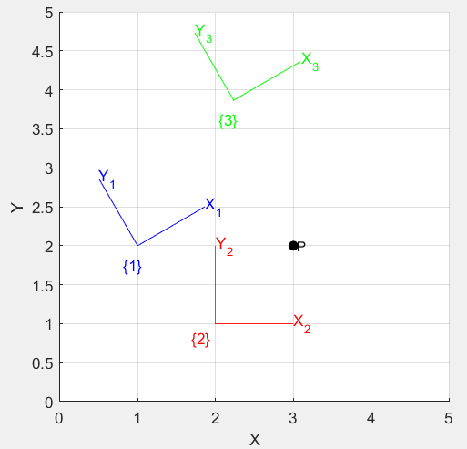
Plotting도 할 수 있다.
plotvol([0 5 0 5]);
trplot2(T1, 'frame', '1', 'color', 'b')
trplot2(T2, 'frame', '2', 'color', 'r')
trplot2(T3, 'frame', '3', 'color', 'g')
World frame에 점 $(3,2)$를 정의하고 plotting하자.
P = [3;2];
plot_point(P, 'label', 'P', 'solid', 'ko');
좌표계 $\{1 \}$에 대한 점의 좌표를 구하고 싶다.
\[{}^0 \textbf{p} = {}^{0}\xi_{1} \cdot {}^1 \textbf{p}\]이를 재배열하여,
\[\begin{align*} {}^1 \textbf{p} &= {}^{1}\xi_{0} \cdot {}^0 \textbf{p} \\ &= ({}^{0}\xi_{1})^{-1} \cdot {}^0 \textbf{p} \\ \end{align*}\]따라서,
P1 = inv(T1) * [P; 1]
P1 =
1.7321
-1.0000
1.0000
여기서는 Euclidean 좌표계를 homogeneous form으로 바꾸어 계산했다. 만약 Euclidean 좌표계를 답을 내고 싶다면,
h2e( inv(T1) * e2h(P) )
ans =
1.7321
-1.0000
e2h는 Euclidean coord.를 homogeneous로 변환. 반대로 변환할 때는 h2e 함수를 사용.